About Our Analysis

Property Analytics uses a cross-sectional factor-based approach to analyse the London real estate market, similar to those widely used in equity market analysis. This methodology allows us to decompose property returns into specific factors that drive market prices.

Factor Model Development

Our model was developed through rigorous statistical analysis of London property transaction data from 1995. We employed multiple regression techniques to identify the key factors that consistently explain variations in property prices across different market cycles.

A Cross-sectional model

Decomposing returns into factors can be done in mainly three ways: a purely statistical approach, time-series regression, and cross-sectional regression. The first one is hard to interpret, and the second one requires knowing the factor returns a priori. The third one is the most powerful and therefore widely used for stocks. All it requires is knowing the characteristics of each property and regressing the prices on those to derive the factor returns. Fortunately, this is very easy for properties where we can use, for example, the number of rooms, but it's somewhat harder for stocks.

Mathematical Model

At each month t, we fit a cross-sectional OLS of log(price/sqm) on property characteristics, each centred on its window mean X̄_j,window — the mean of X_j over the transactions in the rolling 3-month window:

\[ y_i \;=\; \alpha_t \;+\; \sum_{j=1}^{k} \beta_{t,j}\bigl(X_{i,j} - \bar{X}_{j,\text{window}}(t)\bigr) \;+\; \varepsilon_i \]

Centring makes the intercept α_t interpretable as the log-price of the average transaction in the current window. Each β_t,j is the premium paid per unit of characteristic j at time t.

The period-on-period change in quality-adjusted log-price decomposes via a first-order Taylor expansion evaluated at t:

\[ \Delta \hat{y}(t) \;=\; \Delta\alpha_t \;+\; \sum_{j=1}^{k} \Bigl[\underbrace{\beta_{t,j}\,\Delta X_j}_{\text{composition}} \;+\; \underbrace{X_j(t)\,\Delta \beta_{t,j}}_{\text{factor return}} \;-\; \underbrace{\Delta \beta_{t,j}\,\Delta X_j}_{\text{cross term}}\Bigr] \]

The first two terms use current-period weights (β_t, X_t). This is not an exact first-order decomposition of d(β·X) — it over-counts by Δβ·ΔX. We track that cross term explicitly as its own column in factor_returns.csv so the decomposition closes:

• Baseline Market = cumsum of Δα_t + control-dummy contributions + factor composition effects
• Factor j = cumsum of X_j(t) · Δβ_t,j — the market's repricing of characteristic j at the current basket weight
• Cross Term = −cumsum of Σ_j Δβ_t,j·ΔX_j — reconciles the non-exact split

By construction Baseline + Σ Factors + Cross Term exactly equals the cumulative change in ŷ(t). The cross term is usually small in practice (second-order in monthly changes) but is plotted explicitly on the Trends page so you can see the bias it would introduce under a naive current-values split.

Factor Selection Process

We started with a comprehensive set of potential factors and systematically eliminated those with low explanatory power or high correlation with other factors. The final model includes 8 factors that collectively provide a robust framework for understanding London property prices:

• Baseline market return
• Total floor area
• New build premium
• Non-linear floor area
• Number of habitable rooms
• Energy efficiency
• Construction period
• Flat premium

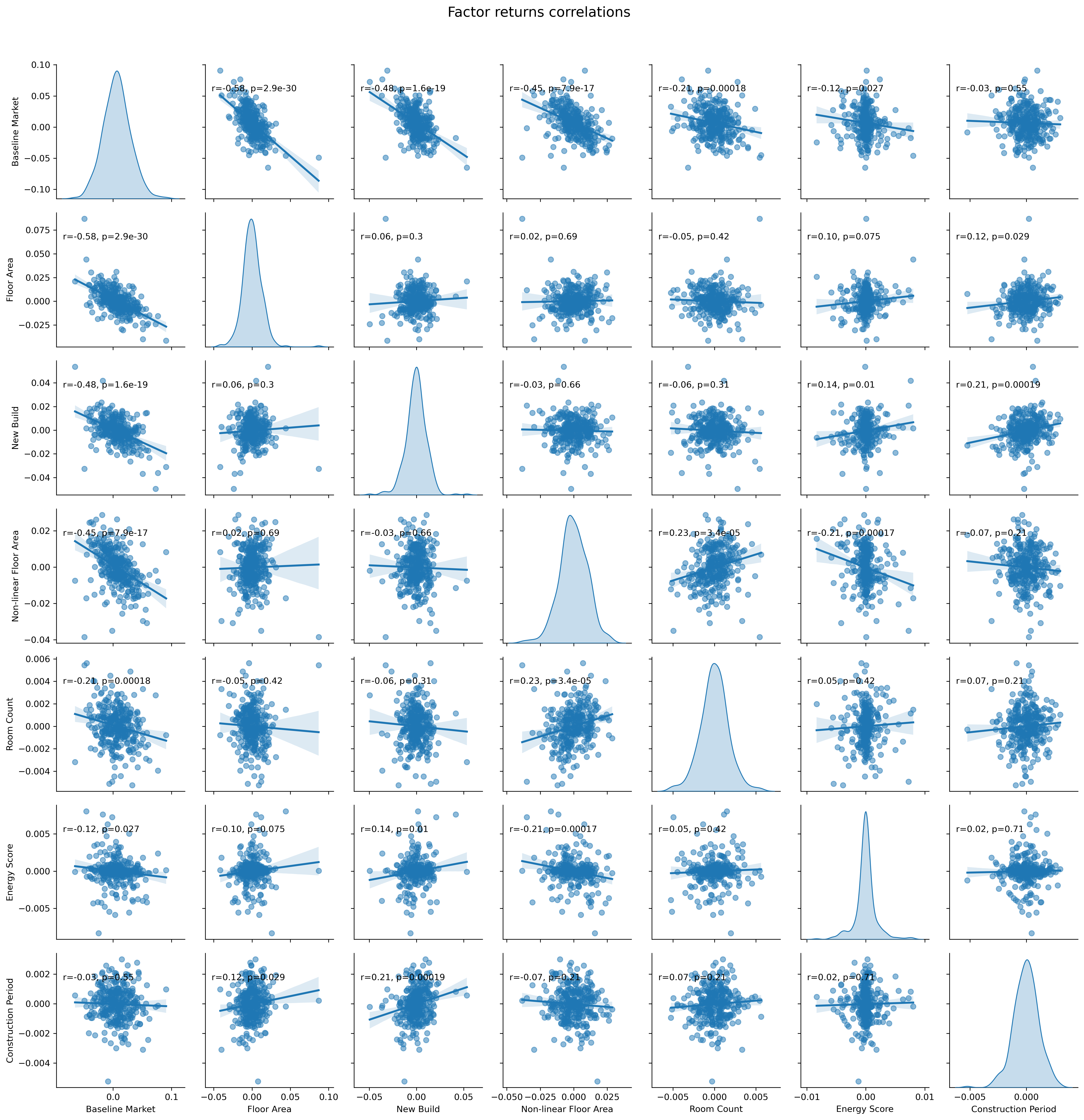
Model Validation

We validate our model using rigorous statistical tests, like ratio between residuals and factor returns, low factor cross-correlations, and low autocorrelations. We also do out-of-sample testing, comparing its predictions against actual market transactions.

A key choice in any hedonic index is the reference basket: the average property whose characteristics are used to translate fitted betas into a price level. We use the actual window mean of each characteristic at time t, so the basket evolves with what is being transacted rather than being frozen on a single representative property.

This decomposition gives two complementary readings per factor: a factor return (X_t·Δβ_j, pure market repricing of characteristic j at today's basket weight) and a composition term (β_t·ΔX_j, the contribution from the basket itself shifting). The composition piece is rolled into Baseline so the factor-return chart stays a clean repricing signal; the Factors page exposes both views per factor.

The basket has shifted materially over 30 years. The charts below track the four dimensions that move the most in the underlying transactions, each expressed as a share of monthly volume:

For reference, the table below summarises the average sold property in four illustrative London market eras:

The 2016 to 2019 period stands out: Help to Buy drove the highest share of new builds and flats ever recorded in London transactions, while EPC standards pushed A/B rated properties from 2% to 15% of sales. Because the regression uses the live basket at each window, these compositional shifts get attributed to the composition term per factor and rolled into Baseline, rather than contaminating the factor returns.

Primary Data Sources

• HM Land Registry Price Paid Data
• Energy Performance Certificate (EPC) data
• Office for National Statistics (ONS) housing data
• London Datastore housing and planning data
• UK House Price Index

Supplementary Data

• Bank of England interest rate data
• UK Census demographic data
• Transport for London accessibility data
• Local planning authority records
• Historical economic indicators